1.I Introduction

Welcome to new set of articles made for computer vision folks. In this article, we will introduce you to processing playing with images. With extensive examples of course, we also will explain the central Python packages you will need for working with images.

This article introduces the basic tools for reading images, converting and scaling images, computing derivatives, plotting or saving results, and so on. We will use these throughout the remainder of our articles journey.

---

1.1 PILLOW vs. OpenCV

If you are using python, you will see that there’re many packages that almost doing the same thing. And here, we will compare between two great packages that are commonly used in image processing and computer vision, OpenCV and PILLOW.

PILLOW	OpenCV
The Python Imaging Library (PIL) provides general image handling and lots of useful basic image operations like resizing, cropping, rotating, color conversion and much more.	OpenCV provides a real-time optimized Computer Vision library, tools, and hardware. It also supports model execution for Machine Learning (ML)
PIL is free and available from https://pillow.readthedocs.io/en/stable/	OpenCV is free and available from https://opencv.org/

Now, let’s warm up with simple snippet, the first thing need to be done is to read an image. And to read an image, use either of the following:

PILLOW	OpenCV
from PIL import Image	from cv2 import imread
pil_im = Image.open('empire.jpg')	cv_im = imread('empire.jpg')

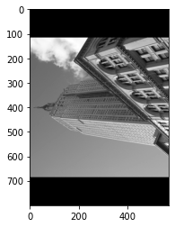
After executing either/both of the code snippets, you will see nothing, because you have loaded it into variables. Now it is the time to show what we have loaded, we will have to do some edits into code snippet we executed above, you can show the image using the following codes:

PILLOW	OpenCV
from PIL import Image	from cv2 import imread
from pylab import imshow, array	from pylab import imshow, array
pil_im = Image.open('empire.jpg')	cv_im = imread('empire.jpg')
pil_im = array(pil_im)	cv_im = array(cv_im)
imshow(pil_im)	imshow(cv_im)
output:	output:

Note that:

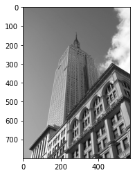
• The returned value in the pil_im variable is a PIL image object. Color conversions are done using the convert() method. To read an image and convert it to grayscale, just add convert('L') like this:
• On the other hand, the returned value in the cv_im is a numpy.ndarray which is considered as a matrix object. So, if you wanted to do any other operation on it, you will back to OpenCV. For example changing the image to grayscale, you will call cv2.cvtColor() and pass the type of conversion needed, such as:

PILLOW	OpenCV
pil_im = pil_im.convert('L')	cv_im = cv2.cvtColor(cv_im, cv2.COLOR_BGR2GRAY)

Hint: You can go back to documentation to find out about the type of conversion you can do with both convert() and cvtColor() methods.

Convert Images to Another Format

Using the save() method, PIL can save images in most image file formats. Here’s an example that takes all image files in a list of filenames (filelist) and converts the images to JPEG files:

PILLOW	OpenCV
pil_im.save('pillow_gray_empire.jpg')	cv2.imwrite('opencv_gray_empire.jpg', cv_im)

The PIL function open() creates a PIL image object and the save() method saves the image to a file with the given filename. The new filename will be the same as the original with the file ending “.jpg” instead.

PIL is smart enough to determine the image format from the file extension. There is a simple check that the file is not already a JPEG file and a message is printed to the console if the conversion fails.

Throughout this book we are going to need lists of images to process. Here’s how you could create a list of filenames of all images in a folder.

For handy operations, let’s write few general lines to get us all the images under directory, just to be able to iterate over and load all of them, here is the code snippet:

Note that: You don’t need to use both of the below lines, either one of them will be more than enough, we need those lines just to save us time for hard coding the image paths.

images = glob.glob("./*.jpg")
print(images)
# --OR--
images = [os.path.join('./', f) for f in os.listdir('./') if f.endswith('.jpg')]
print(images)

Hint: The above code snippet is a general one, it will work for both PILLOW and OpenCV.

Another Hint: The image path might be different if you are using another operating system, and because this was executed on windows, you will find few differences.

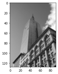
Create Thumbnails

Using PIL to create thumbnails is very simple. The thumbnail() method takes a tuple specifying the new size and converts the image to a thumbnail image with size that fits within the tuple.

In OpenCV it may differ a little, because you will see that resize do the same job with a certain flag cv2.INTER_AREA.

To create a thumbnail with longest side 128 pixels, use the method like this:

PILLOW	OpenCV
pil_im.thumbnail((128,128))	cv_im = cv2.resize(cv_im, (128,128), interpolation=cv2.INTER_AREA)
imshow(pil_im, cmap='gray')	imshow(cv_im, cmap='gray')

Copy and Paste Regions

Cropping a region from an image is done using the crop() method:

PILLOW	OpenCV
box = (20,20,80,100)
region = pil_im.crop(box)	region = cv_im[20:80, 20:100]
imshow(region, cmap='gray')	imshow(region, cmap='gray')

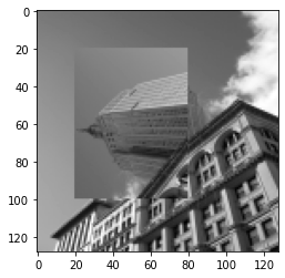
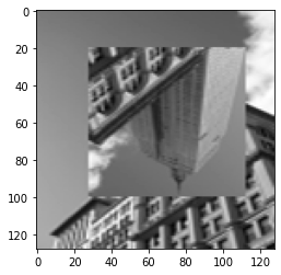
The region is defined by a 4-tuple, where coordinates are (left, upper, right, lower). PIL uses a coordinate system with (0, 0) in the upper left corner. The extracted region can, for example, be rotated and then put back using the paste() method like this:

PILLOW	OpenCV
region = region.transpose(Image.ROTATE_180)	region = cv2.transpose(region)
pil_im.paste(region, box)	cv_im[20:100, 20:80] = region
imshow(pil_im, cmap='gray')	imshow(cv_im, cmap='gray')

Resize and Rotate

To resize an image, call resize() with a tuple giving the new size:

PILLOW	OpenCV
out = pil_im.resize((128,128))	out cv2.resize(cv_im, (128, 128), interpolation=cv2.INTER_AREA)
imshow(out, cmap='gray')	imshow(out, cmap='gray')

In case of OpenCV and you wondered about the flag, visit the documentation to know more about it, but here are few of them.

• CV_INTER_NN (default)
• CV_INTER_LINEAR
• CV_INTER_CUBIC
• CV_INTER_AREA

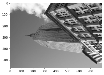
To rotate an image, use counterclockwise angles and rotate() like this:

PILLOW	OpenCV
out = pil_im.rotate(90)	out = cv2.rotate(cv_im, cv2.ROTATE_90_COUNTERCLOCKWISE)
imshow(out, cmap='gray')	imshow(out, cmap='gray')

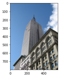
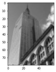
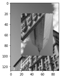
Some examples are shown in Figure 1-1. The leftmost image is the original, followed by a grayscale version, a rotated crop pasted in, and a thumbnail image.

---

1.2 Playing with Images

When working with mathematics and plotting graphs or drawing points, lines, and curves on images, Matplotlib is a good graphics library with much more powerful features than the plotting available in PIL.

Matplotlib produces high-quality figures like many of the illustrations used in this book. Matplotlib’s PyLab interface is the set of functions that allows the user to create plots.

Matplotlib is open source and available freely from https://matplotlib.org/, where detailed documentation and tutorials are available.

Here are some examples showing most of the functions we will need in this book.

Plotting Images, Points, and Lines

Although it is possible to create nice bar plots, pie charts, scatter plots, etc., only a few commands are needed for most computer vision purposes.

Most importantly, we want to be able to show things like interest points, correspondences, and detected objects using points and lines. Here is an example of plotting an image with a few points and a line:

The next code snippet is a general one, where you will put it either you are using PILLOW or OpenCV:

from pylab import *
# some points
x = [100,100,400,400]
y = [200,500,200,500]

PILLOW	OpenCV
from PIL import Image	import cv2
im = array(Image.open('empire.jpg'))	cv_im = imread('empire.jpg')
imshow(im)	imshow(im)

# plot the points with red star-markers
plot(x, y, 'r*') # we will talk about this line next...
# line plot connecting the first two points
plot(x[:2], y[:2])
# add title to the plot
title('Plotting: "empire.jpg"')
# show the plot
show()

Note that: If you are using Jupyter Notebook, please put the whole code above in this section in one code cell to work correctly.

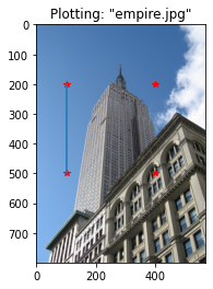
This plots the image, then four points with red star markers at the x and y coordinates given by the x and y lists, and finally draws a line (blue by default) between the two first points in these lists as shown.

The show() command starts the figure GUI and raises the figure windows. This GUI loop blocks your scripts and they are paused until the last figure window is closed.

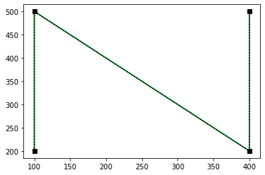
This will give a plot like the one on the right in the plot instead. There are many options for formatting color and styles when plotting.

The most useful are the short commands shown in tables below:

Code	Color
w	White
k	Black
b	Blue
g	Green
r	Red
y	Yellow
c	Cyan
m	Magenta

Code	Mark
.	point mark
o	circle mark
s	square mark
*	star mark
+	plus mark
x	x mark

And you can use them like this:

plot(x,y) # default blue solid line
plot(x,y,'r*') # red star-markers
plot(x,y,'go-') # green line with circle-markers
plot(x,y,'ks:') # black dotted line with square-markers

1.S Summary

Let’s stop over here, because things will be more complicated. In the next article (stay tuned), will contain more complex image processing operations and how to deal with it in both OpenCV and PILLOW.