Introduction

In those series of articles in general, we are going to introduction you to the field of generative modeling. And with that, we shall first look at what it means to say that a model is generative and learn how it differs from the more widely studied discriminative modeling. Then I will introduce the framework and core mathematical ideas that will allow us to structure our general approach to problems that require a generative solution.

What Is Generative Modeling?

We can define a generative model as follows:

A generative model describes how a dataset is generated, in terms of a probabilistic model. By sampling from this model, we are able to generate new data.

Suppose we have a dataset containing images of horses. We may wish to build a model that can generate a new image of a horse that has never existed but still looks real because the model has learned the general rules that govern the appearance of a horse. This is the kind of problem that can be solved using generative modeling. A summary of a typical generative modeling process is shown in the Figure below ⬇️.

First, we require a dataset consisting of many examples of the entity we are trying to generate. This is known as the training data, and one such data point is called an observation.

Generative Versus Discriminative Modeling

As our goal here is to seriously understand what Generative and Discriminative modeling are? It is good to do a comparison to study the difference between both types. If you have studied machine learning, most problems you will have faced will have most likely been discriminative in nature. To understand the difference, let’s look at an example.

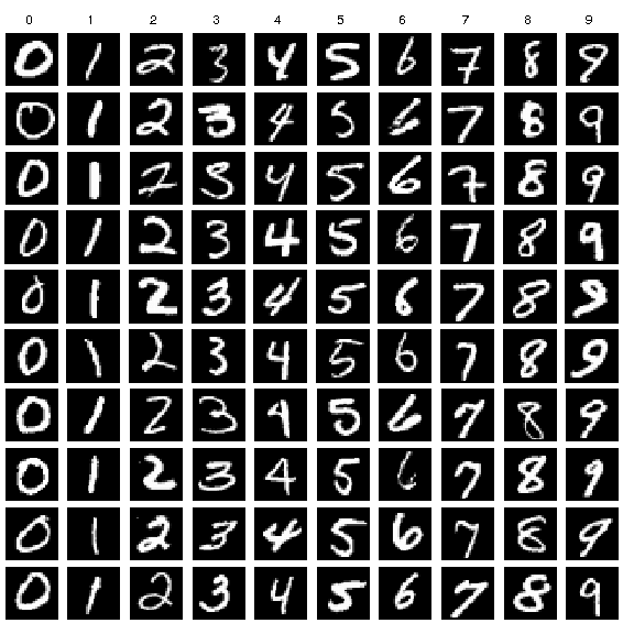
Let’s take an example, let’s assume that we 10 friends, and we know each one handwritings. Not only that, we have a sample data of each one of us writing numbers from 0 to 9.

Discriminative Modeling

We could train a discriminative model to predict if a given number was written by one of us or not. Our model would learn that certain edges, shapes, and textures are more likely to indicate that a written number is by one of us or not,

One key difference is that when performing discriminative modeling, each observation in the training data has a label. For a binary classification problem such as our handwritten discriminator, our handwritten would be labeled 1 and any fake handwrittens number will be labeled with 0. Our model then learns how to discriminate between these two groups and outputs the probability that a new observation has label 1—i.e., that it was written by our group.

For this reason, discriminative modeling is synonymous with supervised learning, or learning a function that maps an input to an output using a labeled dataset.

And the mathematical notation of it, is as follows:

Discriminative modeling estimates p(y

x) which is the probability of a label y given observation x.

Generative Modeling

Generative modeling is usually performed with an unlabeled dataset (as a form of unsupervised learning), though it can also be applied to a labeled dataset to learn how to generate observations from each distinct class.

And the mathematical notation of it, is as follows:

Generative modeling estimates p(x) which is the probability of observing observation x. If the dataset is labeled, we can also build a generative model that estimates the distribution p(x

y).

End of Comparison

In other words, discriminative modeling attempts to estimate the probability that an observation x belongs to category y, whether the categories are either 2 or more.

Generative modeling doesn’t care about labeling observations. Instead, it attempts to estimate the probability of seeing the observation at all.

The key point is that even if we were able to build a perfect discriminative model to identify our handwrittings, it would still have no idea who wrote those numbers. It can only output probabilities against existing images, as this is what it has been trained to do. We would instead need to train a generative model, which can output sets of pixels that have a high chance of belonging to the original training dataset.

Probabilistic Generative Models

Firstly, if you have never studied probability, don’t worry. To build and run many of the deep learning models that we shall see later in this book, it is not essential to have a deep understanding of statistical theory. However, to gain a full appreciation of the history of the task that we are trying to tackle, it’s worth trying to build a generative model that doesn’t rely on deep learning and instead is grounded purely in probabil‐ istic theory. This way, you will have the foundations in place to understand all genera‐ tive models, whether based on deep learning or not, from the same probabilistic standpoint.

As a first step, we shall define four key terms: sample space, density function, paramet‐ ric modeling, and maximum likelihood estimation.

Sample Space. The sample space is the complete set of all values an observation x can take. In our previous example, the sample space consists of all points of latitude and longitude x = (x1, x2) on the world map. For example, x = (31.233334, 30.033333) is a point in the sample space (Cairo).

Probability Density Function. A probability density function (or simply density function), p_{x}, is a function that maps a point x in the sample space to a number between 0 and 1. The summation of the density function over all points in the sample space must equal 1 and can’t exceed 1 at any case, so that it is a welldefined probability distribution. In the world map example, the density function of our model is 0 outside of the orange box and constant inside of the box.

While there is only one true density function pdata that is assumed to have generated the observable dataset, there are infinitely many density functions p_model that we can use to estimate pdata. In order to structure our approach to finding a suitable p_model(X) we can use a technique known as parametric modeling

Parametric Modeling. A parametric model, p_{θ}(x), is a family of density functions that can be described using a finite number of parameters, θ. The family of all possible boxes you could draw on Figure 1-5 is an example of a parametric model. In this case, there are four parameters: the coordinates of the bottomleft (θ1, θ2) and top-right (θ3, θ4) corners of the box. Thus, each density function pθ xin this parametric model (i.e., each box) can be uniquely represented by four numbers, θ = (θ1, θ2, θ3, θ4).

Likelihood. The likelihood ℒ(θ∣x) of a parameter set θ is a function that measures the plausibility of θ, given some observed point x. It is defined as follows: ℒ(θ|x) = p_θ(x) That is, the likelihood of θ given some observed point x is defined to be the value of the density function parameterized by θ, at the point x. If we have a whole dataset X of independent observations then we can write: ℒ θ X = Π x ∈ X pθ x Since this product can be quite computationally difficult to work with, we often use the log-likelihood ℓ instead: ℓ θ X = Σ x ∈ X log pθ x

There are statistical reasons why the likelihood is defined in this way, but it is enough for now to understand why, intuitively, this makes sense. But if you want to learn more about details, will create a small article about the statistical design and will put the link right here.

We are simply defining the likelihood of a set of parameters θ to be equal to the probability of seeing the data under the model parameterized by θ.

In the world map example, an orange box that only covered the left half of the map would have a likelihood of 0—it couldn’t possibly have generated the dataset as we have observed points in the right half of the map. The orange box in Figure 1-5 has a positive likelihood as the density function is positive for all data points under this model.

First Few Lines

Your First Probabilistic Generative Model

Naive Bayes

Back To Your First Few Lines

The Challenges of Generative Modeling

Representation Learning

Summary

Now we came to the end of this article, but we are just starting the series. You will find this article not interesting, but it is important to dig into the various flavors of machine learning. And by that, you learned that a machine learning algorithm is either supervised or unsupervised and either parametric or nonparametric.

Furthermore, we explored exactly what makes these four different groups of algorithms distinct. Until now, we’ve stayed at a conceptual level as you got your bearings in the field as a whole and your place in it.

In the next aricle Building Simple Discriminative Model, you’ll build your first neural network, and all subsequent articles will be project based. So, stay tuned.